

Author: Leon Zhang — Power monitoring and testing equipment team, Baoding Houfeng Trading Co., Ltd., specifying cable test, fault location and high-voltage test instruments for utilities, contractors and industrial plants
Technical review: this guide passed editorial review and was checked against IEEE 1234-2019 and IEC 60502-2:2014 before publication
Last updated: 20 October 2026
Underground cable fault locator types and features decide how many hours a restoration crew spends digging in the wrong place, because a fault that is ranged to ±6 m still has to be pinned to ±0.1 m on the surface before a single sod is lifted. This guide walks through how a locator actually measures distance, which fault classes each method can and cannot see, the specifications that separate a working instrument from an expensive echo machine, and the field setup that turns a reading into a repair. It is written for the engineer specifying equipment for a distribution utility or an industrial network, and for the technician who has to produce a defensible number on the job sheet at two in the morning.
Key Takeaways
- A cable fault locator ranges a fault by time-domain reflectometry: it launches a pulse, times the reflection, and converts elapsed time to distance using the cable’s wave velocity — so the two numbers that decide everything are the sampling rate and the accuracy of the velocity you entered.
- Low-voltage pulse mode handles short circuits, open circuits and low-resistance faults on its own; pulse current and multiple pulse modes add a high-voltage surge generator for high-resistance and flashover faults, and a separate pinpointer is what takes the last step from metres to centimetres.
- The instrument that ranges the fault and the instrument that pinpoints it are different machines: a distance tester answers “how far”, a pinpointer answers “where exactly on the ground”, and IEEE 1234-2019 treats them as two distinct stages of the same job.
- Ranging accuracy is quoted as ±(0.5% of cable length + 1 m) on the HF-CH-204 cable fault locator for cables of 20 m and above, with 0.1 m resolution, a 2 m blind zone, 400 MHz real-time sampling and a 100 km maximum range — figures that only make sense against the cable length you actually test.
What a Cable Fault Locator Actually Measures
A cable fault locator does not see the fault; it sees an echo, and the entire discipline of cable fault location is the discipline of reading that echo correctly under field conditions. The instrument launches a short electrical pulse into the conductor at the test terminal and watches the same conductor for a reflection; every discontinuity — a joint, a termination, a change in cable type, and of course a puncture in the insulation — reflects part of that pulse back toward the instrument. The display is a trace of reflected amplitude against time, and because the pulse travels at a known velocity along the cable, elapsed time converts directly to distance. Double the time, double the distance, and the arithmetic is unforgiving: if the wave velocity you entered is wrong by ten percent, every distance on the trace is wrong by ten percent.
Time-domain reflectometry (TDR) is the measurement principle behind that echo, and it is worth being precise about what it measures: a change in impedance along the line, not a broken conductor as such. A short circuit presents a negative reflection because the impedance collapses toward zero; an open circuit presents a positive reflection because the impedance rises without limit; a high-resistance fault produces a small, easily-missed reflection because the impedance change is partial. That is the whole reason there is more than one ranging mode on a serious locator — the method has to match the impedance change the fault actually produces.
The velocity term deserves respect, because it is the most common source of a wrong answer that looks right. The pulse does not travel at the speed of light; it travels at the velocity of propagation of the cable, typically around half to three-fifths of the speed of light for polymeric-insulation cables, which puts common values in the 150 to 180 m/μs band for XLPE and EPR constructions and lower for impregnated-paper designs. The HF-CH-204 allows the wave velocity to be set from 100 m/μs to 300 m/μs precisely because that spread exists in the real world. The disciplined habit is to calibrate rather than assume: range the cable end-to-end on a healthy phase of known length, read the apparent length, and correct the velocity until the instrument agrees with the tape. Two minutes of calibration removes the single largest error term in the whole measurement.
For example, on a 2.2 km run of 35 kV XLPE cable where the crew assumed 172 m/μs but the actual lay-up and conductor construction gave 160 m/μs, every fault distance read seven percent short — a 150 m error on a fault that was truly 2,150 m away, which is the difference between excavating a road shoulder and excavating a field boundary. Nothing on the trace looked wrong. The number was simply computed with the wrong constant.
One technique quietly improves every reading that follows it: range a healthy phase before you range the faulty one, and keep both traces on screen. The two cables share the same route, the same joints and the same termination, so a divergence between the healthy trace and the faulty trace is the fault, while features common to both are the route. This comparative habit is what turns a single ambiguous blip into a confident answer, and it costs nothing but a mode change. Every underground cable fault locator types and features discussion should start here, because the cheapest accuracy improvement on any instrument is using the cable itself as the reference.

Fault Classes: Five Things That Break a Cable
Before choosing an instrument, classify the fault, because the class — not the cable voltage — decides which ranging method can see it, and a method matched to the wrong class returns a flat trace and a wasted site visit rather than a useful answer. IEEE 1234-2019 organises fault-locating technique selection around exactly this step, and its fault characterization chart exists to keep that mismatch from happening. Five classes cover the overwhelming majority of field work.
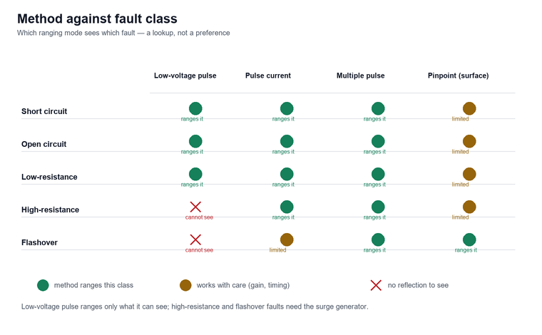
Short circuit means the conductor has a low-resistance path to another conductor or to earth, typically well under a few hundred ohms. The impedance collapse is total, so the reflection is strong and unmistakable, and low-voltage pulse mode ranges it cleanly without any high-voltage source at all. Open circuit — a broken conductor — gives the mirror image: impedance rises to infinity, the reflection is positive and large, and the same low-voltage pulse ranges it. These two are the easy cases, and they are also the cases where the distance answer is trustworthy enough to excavate with confidence after a surface check.
Low-resistance fault sits between those extremes: the insulation is damaged but still passes some current, in the kilohm range or below. The reflection is smaller than a short’s but still well-formed, and low-voltage pulse mode usually still ranges it — the trace just needs a gain increase and a cleaner read. High-resistance fault is the class that breaks cheap equipment: the damaged insulation has carbonised or dried out, and the resistance is high enough that the pulse simply passes the fault without a measurable reflection. The fault has to be forced to break down under a controlled high-voltage surge, which is why pulse current and multiple pulse methods pair the reflectometer with a surge generator. Flashover is the intermittent cousin: the insulation holds at operating voltage but breaks down at some higher voltage, often unpredictably, so the fault only exists during the surge and the method has to catch it while it is there.
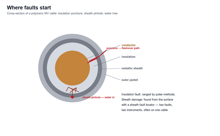
Fault class also interacts with cable construction, and this is where the sheath enters the picture. On a polymeric cable, water ingress through a damaged outer sheath grows water trees in the insulation until the dielectric fails — a slow mechanism that ends in exactly the high-resistance and flashover faults that dominate medium-voltage networks. The insulation fault is ranged with the pulse methods; the sheath damage that caused it is a different measurement on a different instrument, and on long circuits both jobs often need doing.
The causes behind those classes are worth naming, because they tell a buyer which class to expect on their own network. Third-party mechanical damage during excavation is the classic origin of shorts and opens on distribution circuits, and it tends to cluster where other utilities share the trench. Ageing terminations and joints manufactured under time pressure produce the low-resistance faults that appear during routine testing. Water treeing from sheath damage, as above, and simple insulation ageing under sustained thermal and electrical stress produce the high-resistance and flashover classes. A utility whose fault history is dominated by excavation damage needs ranging range and pinpointing robustness; a utility whose history is dominated by ageing insulation needs surge capability and PD-informed prioritisation, which is a different equipment conversation.
| Fault class | Typical origin | Reflection seen by low-voltage pulse | Method that ranges it |
|---|---|---|---|
| Short circuit | Excavation damage, crushed insulation | Strong negative reflection | Low-voltage pulse alone |
| Open circuit | Broken conductor, pulled joint | Strong positive reflection | Low-voltage pulse alone |
| Low-resistance fault | Ageing termination, wet joint | Small but usable reflection | Low-voltage pulse with gain |
| High-resistance fault | Water treeing, carbonised track | No measurable reflection | Pulse current or multiple pulse with surge generator |
| Flashover | Intermittent breakdown under voltage | No reflection between surges | Pulse current or multiple pulse, timed to the arc |
Underground Cable Fault Locator Types and Features
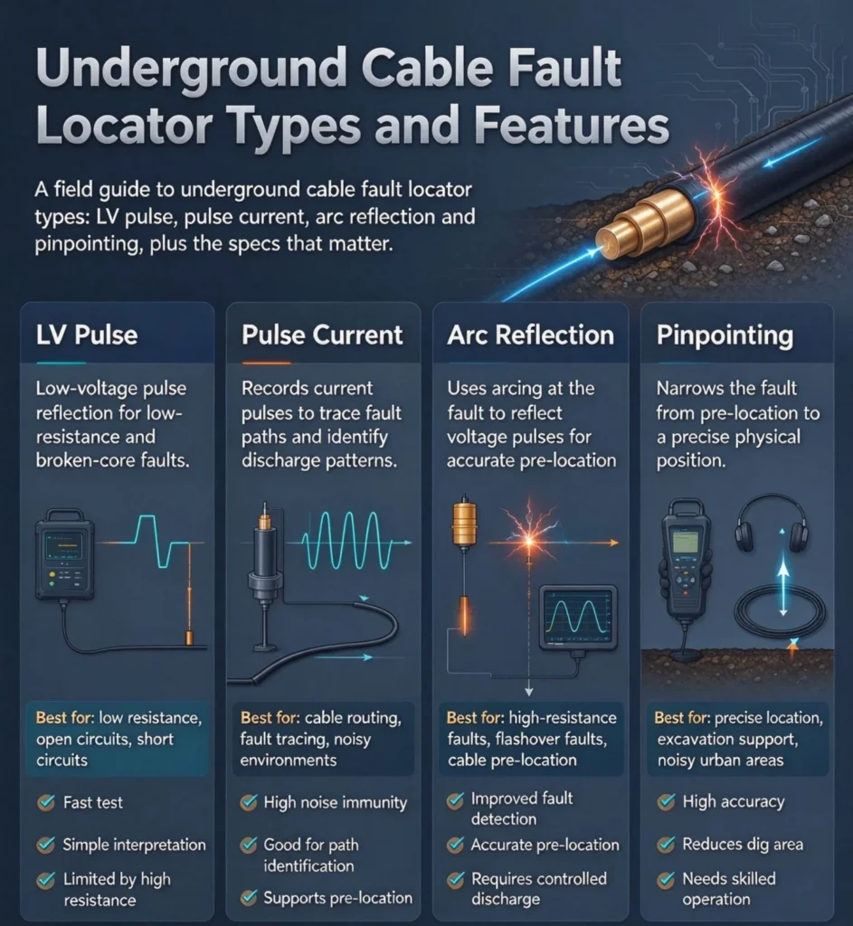
Types, in practice, means two things at once: the ranging modes an instrument supports and the instrument classes that make up a complete fault-location kit, and both matter to a buyer because the modes decide which faults you can range and the kit decides whether you can finish the job.
Low-Voltage Pulse: The Fast, Safe, Limited Mode
Low-voltage pulse mode is the reflectometer working alone, launching a pulse of a few tens of volts — 30 V on the HF-CH-204 — into the de-energised, isolated cable. No high-voltage source, no coupling gear, no special safety perimeter beyond normal isolation and earthing discipline. It ranges short circuits, open circuits, low-resistance faults, and it measures total cable length, finds intermediate joints and T-joints, and calibrates wave velocity. Pulse width is adjustable from 40 ns to 20.5 μs, and that adjustment is not cosmetic: a narrow pulse resolves closely-spaced features and near-end faults but attenuates over distance, while a wide pulse reaches further with coarser detail. The trade is the same one radar and sonar have always made.
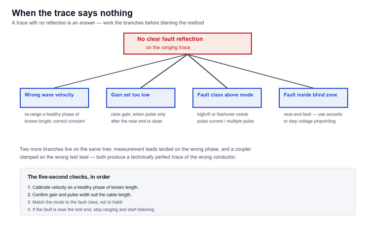
The mode’s ceiling is equally clear. A high-resistance or flashover fault produces no reflection a low-voltage pulse can see, so on a solidly-faulted medium-voltage cable the trace comes back looking like a healthy cable of the right length. Operators new to the work routinely read that as “no fault found” when the truth is “this mode cannot see this class”.
Pulse Current: Where High-Resistance Faults Answer
Pulse current mode adds a high-voltage surge generator and a current coupler. The generator charges the cable and fires a surge that drives the fault into breakdown; the discharge creates a transient current that the coupler — clamped around a test lead rather than connected across the high voltage — picks up and feeds to the reflectometer. The reflection now comes from the arc at the fault, not from an impedance mismatch, and the class of fault that was invisible to the low-voltage pulse becomes locatable. The coupler arrangement matters for safety as much as signal: it gives complete galvanic isolation between the high-voltage circuit and the measurement input.
The price of the capability is the high-voltage perimeter. The cable must be isolated, discharged and earthed at the far end according to the site’s switching plan, the surge generator and its earth become part of the test setup, and the procedure stops being a one-person five-minute job. On the HF-CH-204 this mode also shares the display with the low-voltage trace through a picture-in-picture comparison, which lets the operator confirm that the fault reflection and the end-of-cable reflection agree between methods before anyone trusts the number.
Multiple Pulse: Easier Waveforms, Same Answer
Multiple pulse mode is the current evolution of the secondary-pulse family, and its purpose is waveform readability. The instrument fires a high-voltage pulse that burns the fault into an arc, records a low-voltage pulse trace while the arc is conducting, then records a second trace after the arc extinguishes and the fault returns to high resistance. Overlaying the two traces puts a visible divergence at the fault distance and a clean, short-circuit-style waveform everywhere else — which removes the interpretive burden of hunting a small blip on a raw arc-reflection trace. On difficult faults, that difference is the difference between a confident number and an argument.
The requirement is a multiple-pulse coupler in addition to the surge generator, and the discipline is synchronisation: the arc lasts microseconds, so the low-voltage sampling pulse has to fire inside that window, repeatedly, until a usable pair of traces is captured. Not every shot succeeds, and a crew that has never seen the mode work sometimes concludes the instrument is faulty when it is simply waiting for the right shot.
Pinpointing Modes: Acoustic-Magnetic and Step Voltage
Ranging answers “how far”. Pinpointing answers “where”, and it happens on the ground surface, after the range is known. The workhorse is acoustic-magnetic synchronisation: each surge discharge at the fault produces a thump in the soil and a magnetic field pulse at the same instant; the pinpointer listens for the thump with a ground sensor and watches for the magnetic pulse, then reports the time delay between them. Walk the route, and the delay collapses to zero at the point directly above the fault.
The HF-CH-205 pinpointer implements this with a full-band audio channel from 100 Hz to 1500 Hz, four selectable filter ranges to suppress traffic and machinery noise, at least 80 dB of gain, and a stated pinpointing accuracy of 0.1 m. It adds a magnetic-field-intensity mode for tracing the route and a step-voltage option for the cases where the ground is too noisy or the soil too dry for acoustics. Step voltage works on a different principle: with the fault energised from a high-voltage source, the soil surface above the fault carries a potential gradient, and a probe walking that gradient points at the fault direction. The sheath side of the job uses the same family of methods on the metallic screen, with a stated step-voltage accuracy of 1% (±0.1 mV) at 0.1 mV maximum sensitivity — the working principle behind the HF-CH-208 sheath fault locator, which adds a fault-current mode for sectional positioning and a high-voltage probe mode for trenches and concrete ducts, and the reason a sheath puncture is treated as a fault class no insulation locator can see.
An underground fault locator earns its keep in the last hundred metres, not the first two kilometres. The distance tester narrows the search to a stretch of route; the pinpointer walks that stretch and puts a mark on the ground that an excavator can work to. Treating the two as one instrument is the most common specification error in this category, and it is the reason a “locator” purchase that looks complete on paper still leaves a crew digging a trench along a whole feeder.
Key Specifications, Line by Line
Specification sheets for this category are long, and most of the lines are marketing; five numbers decide whether an underground cable fault locator types and features sheet survives contact with a real feeder, and the rest is ergonomics.
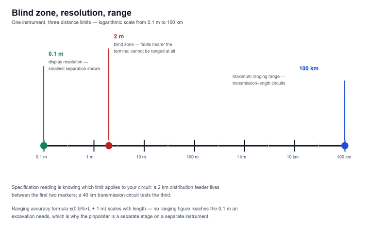
Ranging accuracy is quoted as a formula, not a single figure, and the formula is the specification. The HF-CH-204 states ±(0.5% of cable length + 1 m) for cables of 20 m and above — read that as a scaling error plus a floor: on a 500 m circuit the error budget is ±3.5 m, on a 5 km circuit it is ±26 m, and on a 20 km circuit it is ±101 m. A buyer comparing “accuracy” between two instruments without comparing the formula is comparing nothing. This is also the number that tells you pinpointing is not optional on long circuits: no ranging formula ever gets you to the centimetres an excavator needs.
Resolution and blind zone are different limits and often confused. Resolution is the smallest distance separation the display can show — 0.1 m on the HF-CH-204, which is what lets a closely-spaced joint pair resolve as two reflections rather than one lump. The blind zone is the stretch immediately after the test terminal where the launch pulse has not yet decayed enough for a reflection to be seen — 2 m on the same instrument. A fault inside the blind zone cannot be ranged by pulse at all, and on short service cables into a building, a two-metre blind zone at the test end is exactly where faults live.
Sampling rate sets the finest time resolution and therefore the credibility of the small numbers. Real-time sampling at 400 MHz on the HF-CH-204 means a sample every 2.5 ns; combined with the 0.1 m resolution figure, that is what makes near-end fault work on short cables possible. Equivalent-time sampling at the same headline megahertz is not the same instrument, because it reconstructs the trace from repeated shots rather than capturing the event as it happens.
The display is the specification nobody quotes and everybody uses. An eight-inch screen at 1500 cd/m² on the HF-CH-204 is not a luxury line on a datasheet; it is the difference between reading a cursor position in full sunlight on a road verge and shading the screen with a jacket while a traffic management crew waits. Automatic brightness, colour-coded traces in multiple-pulse mode and a picture-in-picture layout that holds three stored waveforms alongside the live one are all readability features, and readability features are accuracy features when the reading is taken by a tired technician at the end of a night shift.
Maximum range and gain travel together, and both are about the far end of long circuits. A 100 km maximum ranging range covers transmission-length circuits, and the 70 dB adjustable gain range is what keeps a reflection from a 40 km fault above the noise floor. A locator that ranges beautifully to 2 km and gives up at 8 km is a distribution tool being asked to do transmission work.
Wave velocity range, storage and connectivity decide day-to-day usability. The 100 to 300 m/μs velocity setting range covers every cable in service; storage of 100 waveforms with USB export and optional Bluetooth means a crew can compare today’s trace with last year’s on the same circuit, which is how a developing fault gets caught before it operates.
When comparing instruments, ask the questions the sheets do not answer. What is the accuracy formula, at what cable lengths, and is it measured or calculated? Is the sampling real-time or equivalent-time? What is the blind zone at the narrowest pulse width, not the widest? Which accessories does each mode require — coupler, surge generator rating, pulse coupler — and are they in the quoted price or a line item? What is the display legibility in direct sunlight, because every one of these readings is taken outdoors? A vendor who answers those five questions with numbers rather than adjectives is describing an instrument that has been used on real feeders.
| Underground cable fault locator types and features | HF-CH-204 cable fault locator | HF-CH-205 pinpointer | HF-CH-208 sheath fault locator |
|---|---|---|---|
| Job in the kit | Pre-location: distance to fault | Pinpointing: exact point on the ground | Sheath damage on buried cables |
| Method | Low-voltage pulse, pulse current, multiple pulse | Acoustic-magnetic sync, magnetic intensity, step voltage (option) | Step voltage, fault current, HV probe |
| Headline accuracy | ±(0.5% × L + 1 m), L ≥ 20 m | 0.1 m pinpointing | 1% (±0.1 mV) step voltage |
| Resolution / sensitivity | 0.1 m, 2 m blind zone | 0.1 m | 0.1 mV |
| Needs high voltage? | Pulse current and multiple pulse modes need a surge generator | Works from the discharge of the ranging step | HV probe mode up to ±10 kV DC |
| Field kit weight | 2.6 kg main unit | 0.6 kg main unit, 1.4 kg sensor | 0.9 kg receiver |
The Three Stages of Fault Location
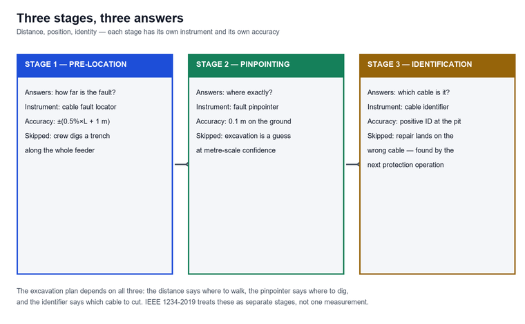
IEEE 1234-2019 frames cable fault location as a staged workflow rather than a single measurement, and the staging is the most useful mental model a buyer can bring to a specification discussion, because skipping a stage means the next one inherits every error the skipped one would have caught.
Stage one is pre-location, and it answers distance. The faulty phase is identified, the fault class is characterised, and the ranging method is chosen to match. The output is a distance from the test terminal plus an uncertainty from the accuracy formula — on a 3 km circuit with the HF-CH-204, a reading of 1,840 m means somewhere within roughly ±10 m of 1,840 m. That number decides which stretch of route gets walked, nothing more.
Stage two is pinpointing, and it answers position on the ground. The route is traced, the pre-located stretch is identified on the surface, and the pinpointer walks it until the acoustic-magnetic delay collapses or the step-voltage gradient points at one spot. The output is a mark and a confidence, and the accuracy figure here — 0.1 m on the HF-CH-205 — is what an excavation is actually planned against.
Stage three is identification and verification, and it is the stage that gets dropped. Before the ground is opened, the cable at the dig point is positively identified, because on a multi-circuit ducted route the pre-located cable is a hypothesis until it is proved. The HF-CH-201 power cable identifier exists for this step, and after excavation the fault is confirmed visually before the repair is closed out — a repair to the wrong cable is discovered by the next operation of the protection, not by the crew that left site.
The records each stage produces are the connective tissue of the whole workflow, and they are what makes the next fault on the same circuit cheaper. A stored trace with its mode, gain, pulse width and velocity constant recorded against the circuit identifier lets the next crew start from a known-good baseline instead of from zero. Over a few years that history becomes the network’s fault memory: which circuits fault repeatedly, which joints were repaired and when, and which sections are living on borrowed time. None of that requires software beyond a folder structure, but it does require the discipline of storing the waveform at the time rather than trusting memory at the next failure.
Field Test Setup and Procedure
The field setup is where a specification becomes a result, and it is remarkably unglamorous, because most bad readings come from the setup rather than from the instrument and the discipline that fixes them is procedural rather than technical. The sequence below is the one that produces a trace a crew can defend.
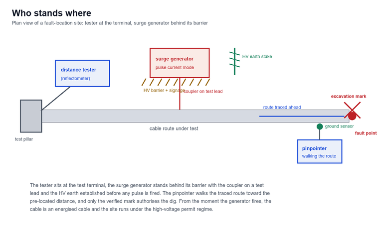
Preparation and isolation. Confirm the circuit is de-energised, isolated, discharged and earthed at both ends under the site switching plan. Identify the faulty phase, and where possible range a healthy phase of the same circuit first to calibrate wave velocity against a known length. Fit the test leads, select the mode, and for pulse current or multiple pulse work, position the surge generator, connect the coupler around a test lead, and establish the HV earth before any pulse is fired.
Choosing the test end is a decision, not an accident of which pillar the van parked at. Test from the end that gives the shortest, cleanest route to the pre-located distance, because every joint and every cable-type change between the test terminal and the fault is another feature on the trace to interpret. Where both ends are accessible, range from both and compare: two independent distances that agree to within their combined error budgets are the strongest evidence a crew can carry into an excavation, and the disagreement itself is diagnostic — a distance that changes with the test end points to a branched or T-jointed section that the route map does not show.
Pre-location. Range the fault in low-voltage pulse mode first even when you expect to need pulse current — the healthy-phase and end-of-cable traces you capture are the comparison references for everything that follows, and the picture-in-picture display is built to hold them. Then move to pulse current or multiple pulse as the fault class requires, capturing both the with-arc and without-arc traces where the mode allows it.
Route tracing and pinpointing. Trace the route from an accessible point toward the pre-located distance, walking the pinpointer along the traced path with the audio filter set to reject the dominant local noise. Mark the point where the acoustic-magnetic delay collapses, verify from a second approach direction, and mark again — two independent marks that agree are worth more than one confident mark.
Verification and records. Identify the cable at the marked point, record the trace, the mode, the velocity constant, the distance and the surface marks in the job sheet, and only then authorise excavation. The stored waveforms — up to 100 on the HF-CH-204, exported over USB — are the evidence that the number was measured rather than estimated.
None of that discipline is instrument work. It is the practice that turns underground cable fault locator types and features into a number a crew can defend, and it is where most avoidable errors live. A safety note belongs in the same breath: the moment a surge generator is connected, the job is a high-voltage test, and the perimeter, earthing, discharging and permit regime that applies to any high-voltage test applies here. The coupler arrangement on the HF-CH-204 isolates the measurement input from the high-voltage circuit, but isolation of an input is not isolation of a site — the cable under surge is an energised cable for the duration of the shot, and the crew’s switching discipline, not the instrument’s safety features, is what keeps it that way in the paperwork and not in the incident report.
For example, a 6/10 kV feeder tripping on a residential circuit ranged at 742 m against a calibrated velocity of 168 m/μs, but the trace’s end-of-cable reflection sat at 812 m where the route map said 800 m — a one-and-a-half percent disagreement that put the fault somewhere near 748 m rather than 742 m. Walking from the pit at 760 m with the pinpointer in band-pass filter, the acoustic delay collapsed at 747.5 m; the excavation found a mechanical-damage puncture at 747.6 m, within the 0.1 m the pinpointer claimed. Two instruments, two stages, one hole.
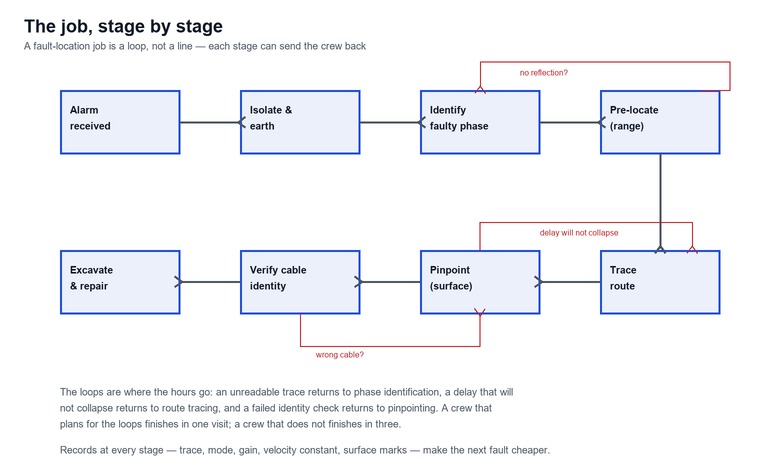
Across fault-location job files kept by our partner service crews, the pattern that separates a one-visit repair from a three-visit repair is almost never the instrument. In the files reviewed, jobs that ranged a healthy phase for velocity calibration before touching the faulty phase finished with a first-dig success rate noticeably higher than jobs that ranged the faulty phase directly, and the failed jobs that did occur clustered on two causes: a velocity constant copied from a previous job on different cable, and a pinpointer walk that started from the test terminal instead of from a known route feature. Neither failure is an instrument failure, and both are invisible on a specification sheet.
Limitations and Boundaries
No locator in this class sees every fault, and the honest specification conversation names the limits before purchase rather than after the first failed job, because the crews that buy on headline numbers are the crews that discover the boundaries on site.
A distance tester cannot pinpoint. Ranging formulas bottom out at metres, and the ±(0.5% of length + 1 m) figure on a 10 km circuit is ±51 m of route to walk. A kit without a pinpointer is a kit that cannot finish, and the missing stage shows up as a trench opened along a feeder rather than at a point.
Blind zones and near-end faults defeat pulse methods. The first 2 m after the test terminal are invisible to the ranging pulse, so a fault in a pillar, a switchgear terminal or the first bend of a service cable cannot be ranged by any pulse method at all — it has to be found by acoustic or step-voltage means with the cable energised from a surge source, a different job with a different safety case.
Dry, rocky or trafficked ground degrades pinpointing. The acoustic channel depends on the discharge sound reaching the sensor through the soil, and frozen ground, compacted rock fill, or a busy road mask the thump. Step voltage and magnetic methods carry the job in those conditions, which is why the HF-CH-205’s multi-mode approach is a feature rather than a luxury.
Intermittent faults may not reproduce on demand. A flashover that breaks down at 18 kV during the fault may hold at 16 kV during the test, and no method forces a fault that will not fire — the technique is simply not applicable to a defect that refuses to break down. Burn-down systems exist for the stubborn residue, and some faults are found by replacing the suspect section: a cost decision, not a measurement one.
Frequently Asked Questions
What are underground cable fault locator types and features in practice?
In practice they are the ranging modes and the kit composition. The modes are low-voltage pulse for shorts, opens and low-resistance faults; pulse current and multiple pulse for high-resistance and flashover faults; and the pinpointing modes — acoustic-magnetic synchronisation and step voltage — that take the search from a ranged distance to a mark on the ground. The kit features that matter are sampling rate, resolution, blind zone, gain, wave velocity range, waveform storage and the accessories each mode demands.
What is the difference between a cable fault locator and a cable fault pinpointer?
A cable fault locator measures distance: it launches a pulse, times the reflection and reports how far the fault is from the test terminal, with an accuracy that scales with cable length. A pinpointer works on the surface after the distance is known, listening for the discharge thump and the magnetic pulse and reporting the delay between them, which collapses to zero directly above the fault. One answers “how far”, the other answers “where exactly”, and IEEE 1234-2019 treats them as separate stages.
Can a low-voltage pulse locator find a high-resistance fault?
Not directly. A high-resistance fault produces an impedance change too small for the launched pulse to see, so the trace looks like a healthy cable. The fault has to be driven into breakdown by a high-voltage surge — which is what pulse current and multiple pulse modes do with a surge generator and a coupler — and only then does the reflection appear. If a low-voltage trace shows nothing suspicious on a cable that is known to be faulty, the fault class is the first suspect, not the instrument.
How accurate is cable fault pre-location?
On the HF-CH-204, ranging accuracy is ±(0.5% of cable length + 1 m) for cables of 20 m and above: about ±3.5 m on a 500 m circuit, ±26 m on 5 km and ±101 m on 20 km. That is pre-location accuracy, and it exists to narrow the search, not to authorise excavation. Pinpointing accuracy is a separate figure — 0.1 m on the HF-CH-205 — and that is the one the excavation is planned against.
What is the blind zone on a cable fault locator, and why does it matter?
The blind zone is the distance immediately after the test terminal where the launch pulse has not decayed enough for a reflection to be detected — 2 m on the HF-CH-204. A fault inside it cannot be ranged by any pulse method, and because services, pillars and switchgear terminations all sit close to a testable end, near-end faults are common in distribution work. They are found by acoustic or step-voltage pinpointing with the cable energised from a surge source.
Do I need a separate sheath fault locator?
If your network is polymeric-insulation cable in wet ground, usually yes. Insulation faults are ranged by the pulse methods, but the sheath puncture that admitted the water is on the metallic screen, and no insulation locator sees it. The HF-CH-208 works from the surface in step voltage, fault current and high-voltage probe modes, with 0.1 mV sensitivity in step voltage mode, and it is what tells a crew whether to dig at the insulation fault or at the sheath damage that caused it.
How many waveforms should a locator store, and why?
Enough to keep a history per circuit. The HF-CH-204 stores 100 waveforms with USB export and optional Bluetooth, which lets a crew compare today’s trace against the same circuit’s trace from a previous visit — the comparison that catches a fault developing between operations. Storage is also the audit trail: a stored trace with its velocity constant and mode recorded is what makes a distance defensible months later when the repair invoice is questioned.
Conclusion
Choosing among underground cable fault locator types and features is really choosing which stages of the job your crews can finish in-house, because an instrument earns its place by turning a protection trip into a distance and only earns trust when the mode matches the fault class, the velocity constant is calibrated rather than assumed, and the distance is finished on the ground with a pinpointer. Specify the modes your fault statistics demand, read accuracy as a formula rather than a headline, and budget for the pinpointing and identification stages as separate instruments. For help matching a locator set to your cable list and fault history, contact us with the voltage classes, typical circuit lengths and fault classes you work with, and we will map the cable tester range — including the HF-CH-204 cable fault locator, the HF-CH-205 pinpointer, the HF-CH-208 sheath fault locator and the HF-CH-201 power cable identifier — to the stages your crews actually perform.
References and Technical Sources
- IEEE, IEEE Guide for Fault-Locating Techniques on Shielded Power Cable Systems, IEEE 1234-2019, published 28 June 2019, superseding IEEE 1234-2007 — the staged pre-location and pinpointing workflow, the fault characterization chart that drives method selection, and the limitations of each technique. standards.ieee.org
- IEC, Power cables with extruded insulation and their accessories for rated voltages above 1 kV (Um = 1,2 kV) up to 30 kV (Um = 36 kV) — Part 2: Cables for rated voltages from 6 kV (Um = 7,2 kV) up to 30 kV (Um = 36 kV), IEC 60502-2:2014, the construction and test basis for the medium-voltage polymeric cables whose insulation and sheath faults this equipment locates. iec.ch
- OSHA, Electrical — Overview, the US Occupational Safety and Health Administration reference for electrical workplace hazards and the safe-work practices that apply whenever a surge generator is connected to an isolated cable. osha.gov
- NIST, Applied Electrical Metrology Group, the US National Institute of Standards and Technology calibration programme for AC and DC voltage, current, phase and power, the traceability anchor behind instrument accuracy claims. nist.gov
- Houfeng, HF-CH-204 Cable Fault Locator — technical specifications, the source of the 30 V low-voltage pulse output, 40 ns to 20.5 μs pulse width, 400 MHz real-time sampling, 0.1 m resolution, 2 m blind zone, 70 dB gain, 100 km range and ±(0.5% × L + 1 m) accuracy figures quoted above. monitor-test.com
- Houfeng, HF-CH-205 Cable Fault Pinpointer — technical specifications, the source of the acoustic-magnetic synchronisation method, the 100 Hz to 1500 Hz audio channel with four filter ranges, the 80 dB gain and the 0.1 m pinpointing accuracy quoted above. monitor-test.com